Ten armed testbed for the Bandit problem with C#
I'm continuing my attempt to reproduce examples from Reinforcement Learning: An Introduction book using C#.
In a previous post I reproduced the tic-tac-toe example with some improvements and clarification with respect to the original text. I think it's worth taking a look at it.
Today I'm reproducing the ten armed testbed for the Bandit problem, in particular I want to reproduce the two graphs showing the average reward improvements and the selection rate of the best arm.
The problem, as stated in the book is the following:
You are faced repeatedly with a choice among k different options, or actions. After each choice you receive a numerical reward chosen from a stationary probability distribution that depends on the action you selected. Your objective is to maximize the expected total reward over some time period, for example, over 1000 action selections, or time steps.
10 armed testbed
One key point to understand to follow the ten armed (k=10) testbed is that the total reward is never computed nor analized in the example itself. The underlying intuition is that we want to find the best action available and select that action as much as possible. Ideally everytime. By being able to select the best action, we will automatically optimize the total reward.
Once selected the value of k=10, we have to define the probability distribution for each action. That is done by using a normal distribution with mean=0 and variance=1, we pick 10 samples from this distribution and each sample will be the mean value of a normal distribution with variable=1. We end up with an array of 10 normal distributions, each time we select action i we will pick the i-th distribution and get a sample value from that distribution.
Given that we don't know the probability distribution assigned to each action we have to base our strategies on estimates values. Each time we select an action, we get an actual reward value and we can improve our estimate for that action. We iterate this process trying to improve our estimates. We start with an estimate of zero for all actions. Each of these selection and update of estimates is called a step. A round comprises multiple steps. In the example provided in the book, we found 2000 rounds of 1000 step each.
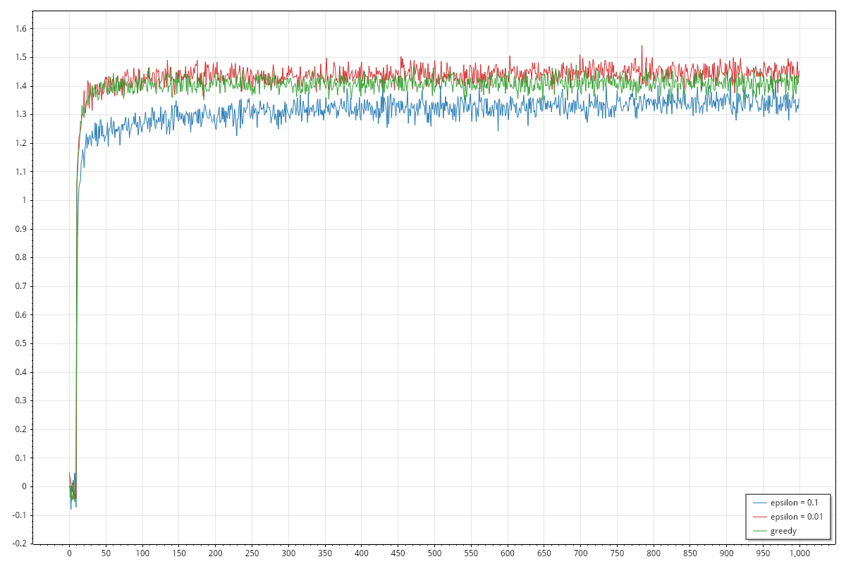
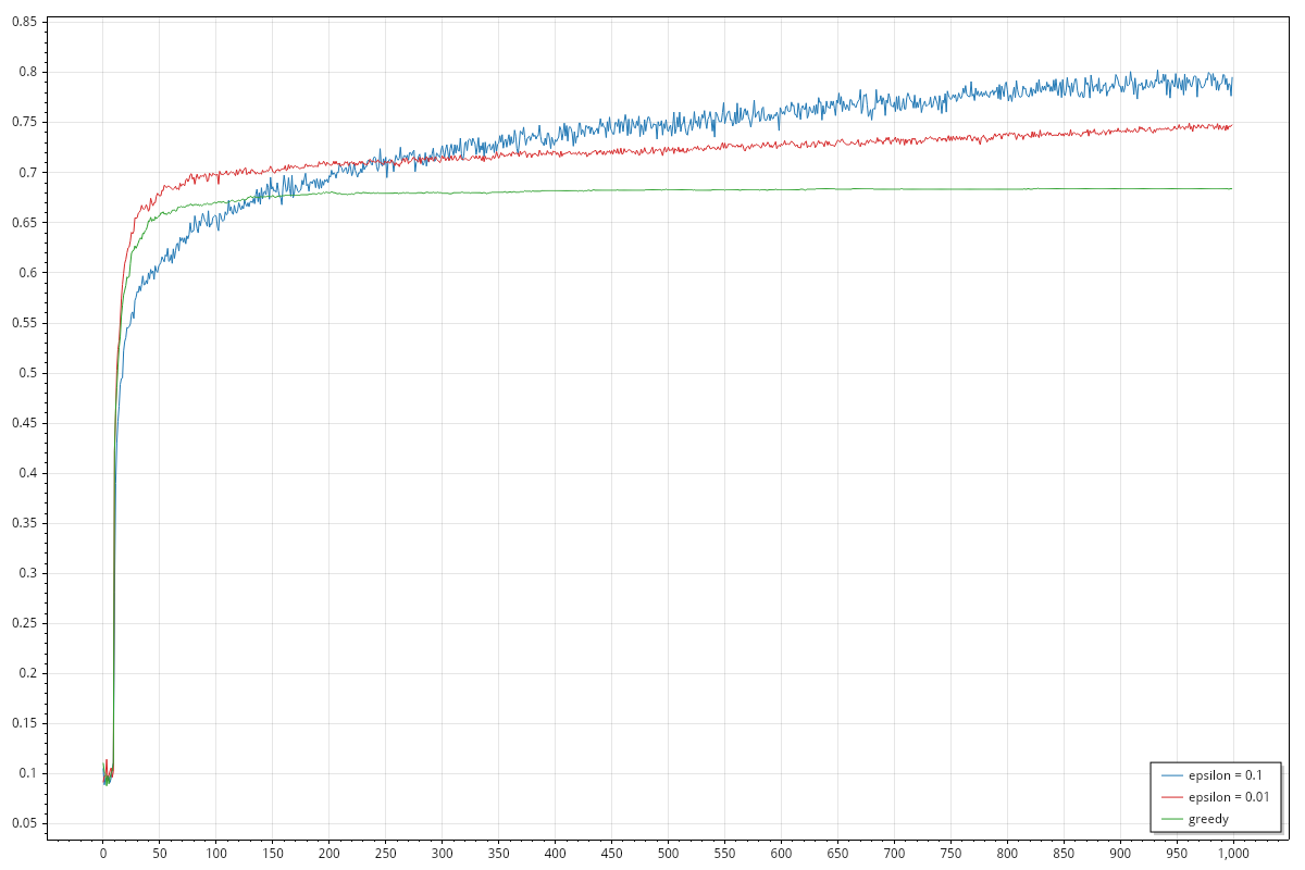
To produce the graphs presented in the book we need to compute:
- for each step, the average reward over the different rounds. For each round, we keep track of reward of step
i. At the end we sum all rewards and we divide by the number of rounds. - for each step, the best arm selection rate. For each step of each round, we keep track of how many times we selected the best action. At the end we sum all values and we divide by the number of rounds. Please remember that we know which arm is best, because we are creating the distributions for each arm. This information cannot be used during the learning process but we can use it to evaluate performances on the testbed.
One point that remains to define is how we select the action. It is evident that we would like to try all of them multiple times so that we can build a reasonable estimate of the value of each action. For example we could select each action in a round-robin fashion and repeat until we complete all steps. This would give us a uniform approach for updating the estimated values, however the best action will be selected roughly 1/k times, in our case corresponding to 10% of the times. That is not very good for the overall performance of the round.
The books suggests three different strategies:
- greedy: we always select the action with the best estimate
- -greedy: on a subset of cases we select a random action, on the remaining ones we select the best strategy:
- 10% of the selections is random (=0.1)
- 1% of the selections is random (=0.01)
Ties are resolved by picking any of the actions with the same expected reward. We already noted that on each step we perform a selection and an update of the estimates. This is true regardless of the strategy, in the tic-tac-toe example we saw that we learned only when the action was selected based on the value table but not when selected randomly. This is not the case here where learning when selecting randomly is the very base for actual improvements.
Greedy strategy
Let's consider for a moment how the greedy behaves on some cases.
We are at step 0, all estimates are 0 so we need to pick a random action between 0-9. Let's say we pick 0:
- if the actual reward is negative, the estimate for 0 will become negative and we won't select 0 in the next step
- if the actual reward is positive, the estimate for 0 will be positive and we will select 0 in the next step. Actually we will continue to select 0 until the estimate become 0 or less. If it is 0, depending on how the tie is resolved we might continue with 0.
From this it's clear that if 0 is not optimal we might end up stuck with 0 for several steps until we are able to evaluate another action.
An observation that we could make is that we could force the greedy strategy to test at least once each action by starting with a default estimate of double.MaxValue. We know that the reward for all actions will be lower than double.MaxValue so at the first 10 steps all actions will be tested, afterwards we will continue with the action that performed the best on the first 10 steps.
-greedy strategy
With the -greedy strategy we are never sure if we are picking the best action, according to our current knowledge, or a random one. However then random one will give us opportunities to improve our estimates.
An improvement over this strategy could be to make smaller as we progress further into our round. The more steps we perform, the better the estimates we have, the lesser need for exploration we have.
Some additional comments
The book notes (bold is mine):
The advantage of -greedy over greedy methods depends on the task. For example, suppose the reward variance had been larger, say 10 instead of 1. With noisier rewards it takes more exploration to find the optimal action, and -greedy methods should fare even better relative to the greedy method. On the other hand, if the reward variances were zero, then the greedy method would know the true value of each action after trying it once. In this case the greedy method might actually perform best because it would soon find the optimal action and then never explore. But even in the deterministic case there is a large advantage to exploring if we weaken some of the other assumptions.
I want to comment on the bold section, because I don't fully agree with what is said there. Let's consider for a moment a ten armed testbed which actions have stationary rewards as [0.05 0.1 0.2 0.3 0.4 0.5 0.7 0.8 0.9] and let's think how the greedy performs.
Given that:
- estimate won't change once updated
- we start with all estimates equal to
0 - we always select the best
the first action selected will change its estimate to a value greater than 0 and it will always be selected without any further exploration. This is a rather artificial example however what is true is that the greedy strategy will always select an action with positive reward once it has found any.
So when the greedy strategy will indeed find the best arm in the stationary case? One case is when the best arm is the only one with a positive reward. Another one is when all arms have negative reward because it will pick one by one all of them on the first steps. Since in case of ties there is some randomization at play, the greedy strategy can select the best arm in other cases.
Different result can be obtained if we change the initial estimate of the actions. Again selecting double.MaxValue as default instead of 0 would force the greedy strategy to select at least once all the arm and then know exactly which one is the best and continue with that.
Code
I implemented of all this in the https://github.com/davidelettieri/sutton-barto-reinforcement-learning repo. I think I left enough comments to allow an easy read of the code, if that's not the case please contact me I'll be happy to add more or explain better if needed.
The graphs are implemented using https://scottplot.net/, you might need to install additional packages, please follow the documentation for more details. On my Fedora 42, at the time of writing, the code works as it is and produce the following graphs:
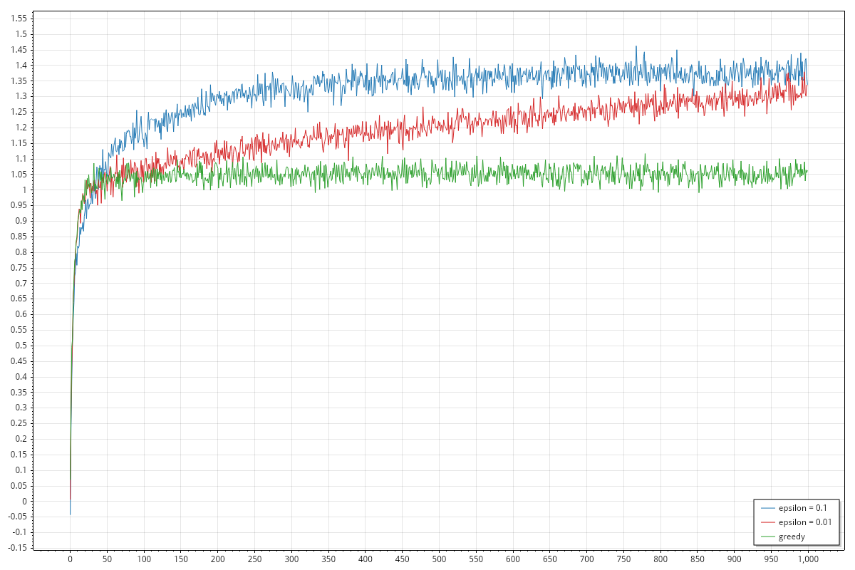
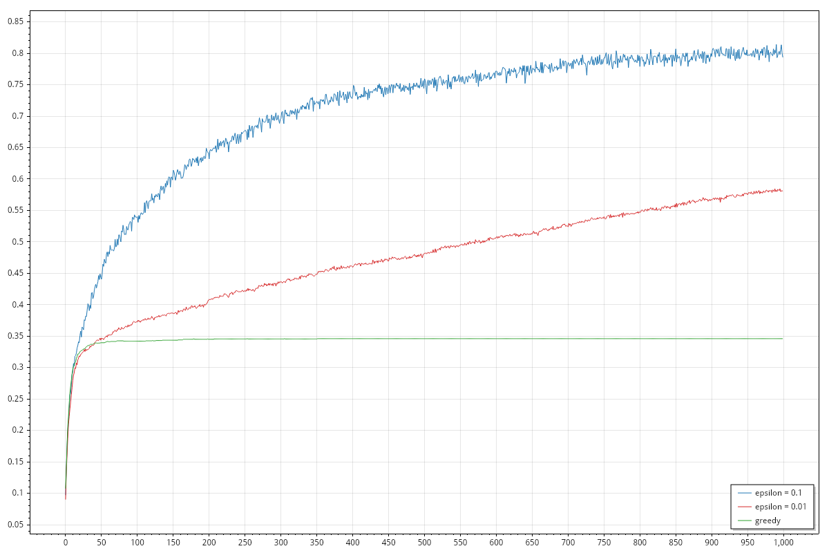
Initializing default estimates to double.MaxValue
When I wrote all of this, I didn't read paragraph 2.6 and I thought that the dependance on the default estimate should have been discussed already. The authors of the book disagree on this and discussed right afterwards in 2.6 Optimistic Initial Values. I, of course, recommend to read the book which is available for free here.
As noted above a couple of times, setting the default estimate to double.MaxValue will force exploration at initial steps for all strategies. The performance of the average reward improves for all strategies, possibly excluding the initial exploration which is quite visible on the graph as brief (10 steps) almost horizontal progress on the three lines. It is noticeable also how the three strategies behave almost with the same performance on the average reward. The graph for the best arm selection rate is rather different from the previous case, showing again more similaties between the three strategies.