Multi armed bandit exercise 2.5 with C#

May 1, 2025 · 5 min read

Recently I tried to code the 10 armed testbed example from chapter 2 of Sutton and Barto Reinforcement Learning: an introduction book.

The chapter continues introducing new theory elements and strategies to improve the approach shown in the 10 armed example. In particular, one of the points is about non-stationary problems.

The 10 armed testbed was a stationary problem, the probability distributions of the different actions don't change over time. If you remember the sample, at the beginning of the round we computed 10 random values, those values are then used to be the mean of a normal distribution from which we will pick the rewards at each step. The constant part is that this normal distributions don't change from a step to another, they stay the same for the whole round execution.

The focus of the exercise is to understand how the estimated reward computation impacts the performance of the $\epsilon$ -greedy strategy. In the 10 armed testbed, the estimate reward was computed averaging the rewards obtained from each action when selected. Note that this approach consider each reward with the same relative value, however in a non-stationary problem, where probability distributions change over time we would like to give more weight or importance to more recent rewards because they represent more realistically the current distribution the reward is generated from.

The text of the exercise is

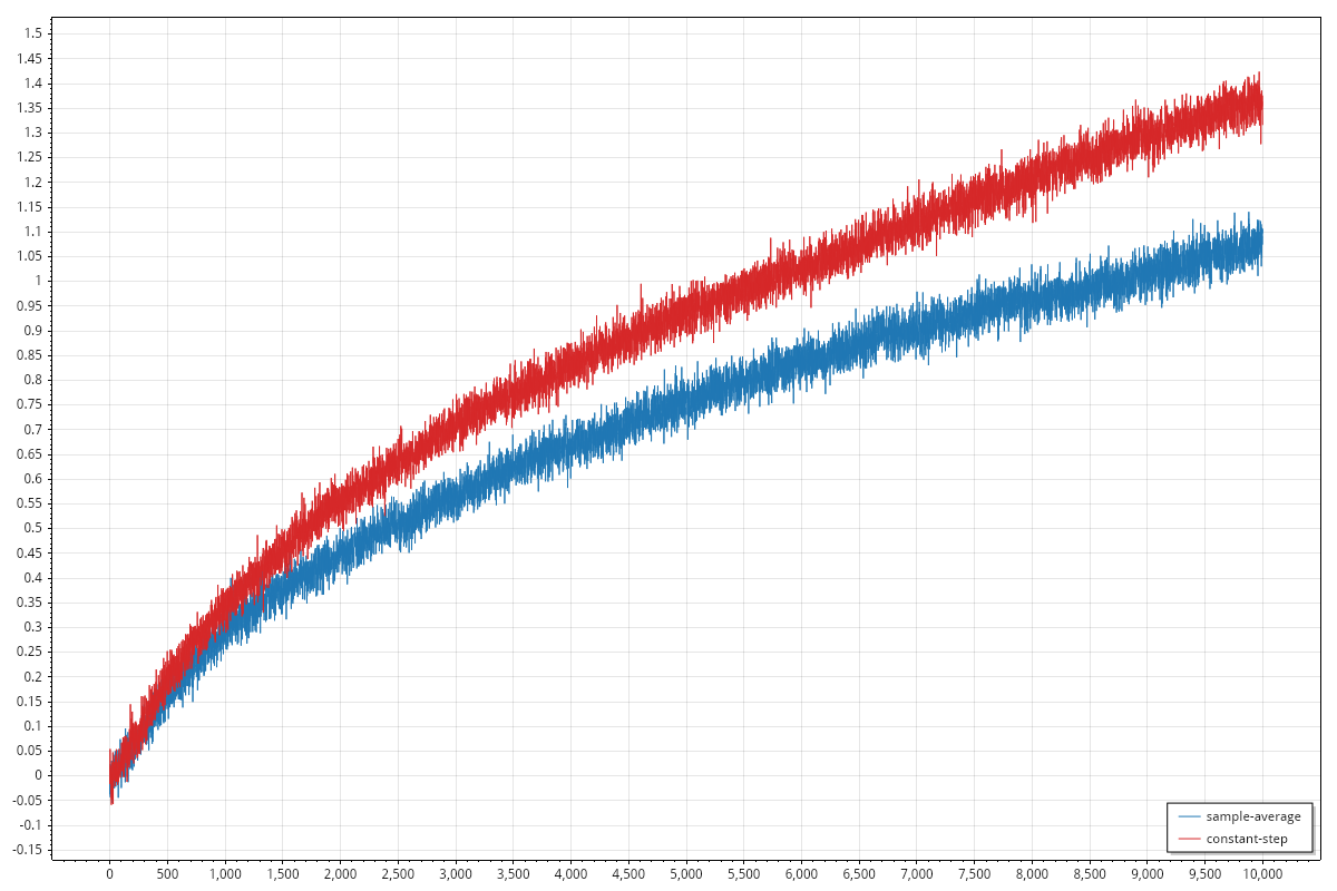
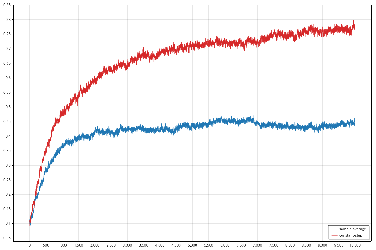
Design and conduct an experiment to demonstrate the difficulties that sample-average methods have for nonstationary problems. Use a modified version of the 10-armed testbed in which all the $q_{*}(a)$ start out equal and then take independent random walks (say by adding a normally distributed increment with mean 0 and standard deviation 0.01 to all the $q_{*}(a)$ on each step). Prepare plots like Figure 2.2 for an action-value method using sample averages, incrementally computed, and another action-value method using a constant step-size parameter, $\alpha$ = 0.1. Use $\epsilon = 0.1$ and longer runs, say of 10,000 steps.

Figure 2.2 refers to the average reward graph and the best arm selection rate graph, the same graphs I produced in the previous post. The $\epsilon=0.1$ refers to the $\epsilon$ -greedy strategy to be used, both in the case of sample averages and in the constant step-size parameter.

The reward estimation formula

The sample average estimation can be naively computed by keeping track of all the rewards for an action and compute the average. However, as the book describes clearly, we can compute the average only by using the current reward, the previous estimate and the number of times the action has been selected. With this approach we have a computational advantage since we don't need to store the rewards for all steps and we need just a few operations to compute the new estimate.

If we denote the estimate at $i$ th as $Q_i$ , the reward as $R_i$ then the formula is:

Q_{n+1} = Q_n + \frac{1}{n}[R_n-Q_n]

Once we have this we can also see how the estimate is computed with constant-step size parameter $\alpha$ :

Q_{n+1} = Q_n + \alpha[R_n-Q_n]

The two formulas are almost the same, the difference $R_n-Q_n$ is multiplied by $1/n$ in one case and by a constant value $\alpha$ in the other.

The implementation

If you checked the previous example I implemented you'll see that the code is mostly the same. I have to support:

non-stationary rewards distributions
different strategies to compute the estimate reward

I don't want to make the previous example too complex and add abstractions to plug in different implementation just to not duplicate code. For both examples I want an easy to follow, low abstraction implementation that I can understand easily in a year from now when all the context I have is lost. However I need to be able to plug in two different strategies for estimate computation, so in that case only I'll use some kind of abstraction:

delegate double UpdateEstimatedReward(double currentEstimatedReward, double reward, int armSelectedCount);

A delegate to capture the function signature of the update formula. The armSelectedCount parameter (I couldn't think of a better name) correspond to the $n$ of the formulas we have above.

And the two formulas translate to

UpdateEstimatedReward sampleAverage = (currentEstimatedReward, reward, armSelectedCount) =>
    currentEstimatedReward + (reward - currentEstimatedReward) / armSelectedCount;

UpdateEstimatedReward constantStepSize(double alpha)
    => (currentEstimatedReward, reward, _) =>
        currentEstimatedReward + alpha * (reward - currentEstimatedReward);

The sampleAverage is just an instance of the delegate while the constantStepSize is a function producing an instance of the delegate. That's because we have the $\alpha$ parameter that needs to be fixed in order to have a concrete update formula. Note also that the third parameter, armSelectedCount, is ignored in the constantStepSize definition.

Regarding the non-stationary part, the exercise text says that we start with equal $q_*(a)$ and the all of them take independent random walks. In the ten armed testbed example, the reward for each actions was a distribution, should be the same here? We have a distribution with variating mean or we should just pick $q_*(a)$ as reward for any step given that it is already changing? I do not know to be honest what the expected approach here, my decision was to go with distributions with changing mean value.

In order to implement correctly the best arm selection rate we have to notice that the best arm is not defined once at beginning but at each step we could end up with a different best arm so we need to compute which one is the best again.

The reward estimation formula​

The implementation​

The reward estimation formula

The implementation